This blog is intended as a home to some musings about M&E, the challenges that I face as an evaluator and the work that I do in the field of M&E.Often times what I post here is in response to a particularly thought-provoking conversation or piece of reading. This is my space to "Pause and Reflect".
Thursday, March 21, 2024
A visualization on statistics choices
Thursday, July 21, 2011
SPSS, PASW and PSPP
PSPP is a program for statistical analysis of sampled data. It is particularly suited to the analysis and manipulation of very large data sets. In addition to statistical hypothesis tests such as t-tests, analysis of variance and non-parametric tests, PSPP can also perform linear regression and is a very powerful tool for recoding and sorting of data and for calculating metrics such as skewness and kurtosis.PSPP is designed as a Free replacement for SPSS. That is to say, it behaves as experienced SPSS users would expect, and their system files and syntax files can be used in PSPP with little or no modification, and will produce similar results.
PSPP supports numeric variables and string variables up to 32767 bytes long. Variable names may be up to 255 bytes in length. There are no artificial limits on the number of variables or cases. In a few instances, the default behaviour of PSPP differs where the developers believe enhancements are desirable or it makes sense to do so, but this can be overridden by the user if desired.
I will give it a test drive an let you know what I think!
PS. to all the "pointy-heads": In the right margin of my blog you will find a link to a repository of SPSS sample syntax!
Wednesday, May 25, 2011
Cohen's d and Effect Size
There are a couple of different ways of calculating an effect size.
r which is the correlation coefficient or R² which is the coefficient of determination
Eta squared ή²
Cohen’s d
This time, I will focus on Cohen’s d.
If you did a t-test, it’s usually a good idea to calculate cohen’s d.
Cohen's d is an appropriate effect size for the comparison between two means. It indicates the standardized difference between two means, and expresses this difference in standard deviation units. The formula for calculating d when you did a paired sample t test is:
Cohen’s d = Mean difference
Standard deviation
If you have two separate groups (in other words you conducted an independent sample t test), you use the pooled standard deviation instead of the standard deviation.
If Cohen’s d is bigger than 1, the difference between the two means is larger than one standard deviation, anything larger than 2 means that the difference is larger than two standard deviations. It is seldom that we get such big effect sizes with the kinds of programmes that I evaluate, so the following rule of thumb applies:
A d value between 0 to 0.3 is a small effect size, if it is between 0.3 and 0.6 it is a moderate effect size, and an effect size bigger than 0.6 is a large effect size.
Here is an example:
Kids wrote a grade 12 exam, then completed a programme that provides additional compensatory education, and then they rewrite the grade 12 exam. Below is a table that compares the Maths mark prior to the programme, to the Maths mark after the programme.
The result is statistically significant (see the last column, p < .000). The learners' results, on average, improved with about 9.9% (Mean difference is indicated in the “mean” column. Usually such a result is indicated as follow:
t (54) = 6.852; p < .000
To calculate Cohen’s d, we divide the mean difference by the standard deviation
d = mean difference/ standard deviation = 9.98148 / 10.70442 = 0.932
0.932 is larger than 0.6 so this can be classified as a large difference. In fact it is close to 1, which means that this programme probably helped the learners, on average, to improve their marks with about 1 standard deviation. That is amazing!
Monday, May 23, 2011
Means and p values.
In the picture below, the mean age at which these kids first drank alcohol, was around age 14. But there are kids who started earlier, and some who started later.
When comparing two means, it is important to determine whether the two distributions differ so much, that it is unlikely that they are both from the same bigger population.
If they differ, the null hypothesis is rejected. If they don’t differ, the alternative hypothesis is rejected.
Notice: although the means differ in B, the overlap in distributions is quite large.
Depending on the scale of the data (nominal, ordinal, interval or ratio) the properties of the distributions (normally distributed or not) and the kind of comparison that’s required (i.e. two independent groups e.g. boys and girls; or two measures for the same group e.g. average for boys before the programme, and after the programme) different statistics may be used.
Usually, we do a t test which yields a t statistic or an ANOVA which yields an F statistic, or their non-paramatric equivalents – the Mann Whitney or Kruskall Wallis test. Because it isn’t very easy to off- hand know if a t of 112 is good or bad, these statistics are converted to a p value (probability value) which indicates how probable it is that the null hypothesis is true.
If the p value is smaller than <0.05, the null hypothesis is rejected – there is only a 5% chance that the two distributions are the same.
Just look carefully at that criterion: p values of 0.5 (50%) and 0.06 (6%) are bigger than 0.05, the null hypothesis will be accepted. A p value 0.045 (4.5%), or any value such as p < 0.000, is smaller than 0.05 and would therefore mean the null hypothesis should be rejected - in other words, the two means differ statistically significantly.
A cut off of p = 0.05 is conventional, but a p of 0.1 (10%) or 0.001 (1%) is sometimes used as a cut-off criterion (depending on the likelihood of Type I and Type II errors)
A result like the one below means:
t (163) = -2.68, p < .05
The t statistic for the means calculated from two groups with 163 cases is -2.68, and is statistically significant at the 5% level.
F (2, 1015) = 111.286, < .001
The F statistic, for a sample of 1015 cases with 2 degrees of freedom (i.e. three groups) is 111.286 and is statistically significant at the 1% level.
The smaller the p value is, the happier you should be – because it means that you will have something interesting to report on!
Monday, March 07, 2011
Specificity and Sensitivity in tests
If your test is highly specific, a low score will be able to identify everyone that requires remediation. - A lack of specificity indicates that some kids who require remediation are not identified.
If your test is highly sensitive, then a high score will clearly exclude anyone that does not need remediation.
SPIN and SNOUT are commonly used mnemonics which helps to remind us ofthe disticntion: A highly SPecific test, when Positive, rules IN disease (SP-P-IN), and a highly 'SeNsitive' test, when Negative rules OUT disease (SN-N-OUT)
Monday, November 12, 2007
Probability Sampling Approaches
Probability sampling approaches allow you to generalize to the full population, since it ensures that special random characteristics are likely to be distributed evenly across the units included and excluded in / from the sample. It therefore is likely to yield a less biased sample and the results could be said to apply to the full population (if the appropriate sample size was selected). Different kinds of probability sampling approaches are possible.
The figures below demonstrate the different approaches. Assume each number is a unique member of the population, assume that each group consists of discreet mutually exclusive members of the population (In columns) and assume that each cluster (delineated by a block) is a group of members in the same geographic area.
With simple random sampling the sample is selected from the whole population using a table of numbers. Note that this does not necessarily ensure balanced representation amongst different groups.
With stratified random sampling, a set number of participants from each group can be selected. Note that this does not necessarily ensure that the most economical approach is used. In the example some cases from almost all of the geographic clusters are included.
With cluster sampling, a set number of clusters are randomly selected (in this case 4) with a set number of randomly selected units within each cluster (in this case 5). Although this will be more economical in terms of fieldwork costs because travel to different clusters have been limited, it does not necessarily guarantee equal representation of groups.
With systematic sampling, a set pattern is systematically applied to select participants. In the case of the example above, every 11th member of the population were selected. Note that it did not require a random table of numbers, but were still subject to the same limitations as the simple random sample.
Type of Probability Samples | When is it applicable | Drawbacks |
Simple Random Sampling (I.e.randomly select 50 schools off a list with all schools in the country) | It is ideal for statistical purposes | · It may be difficult to achieve in practice · It requires a precise list of the whole population · It is costly to conduct as those sampled may be spread over a wide area. |
Stratified Random Sampling (I.e. Randomly select 50 schools per strata such as province) | · It ensures better coverage of the population than simple random sampling. · It is administratively more convenient to stratify a sample – interviewers can be specifically trained to manage particular strata (e.g. age, gender, ethnic or language groups). | · Difficulty in identifying appropriate strata. · More complex to organize and analyse results |
Cluster Sampling (I.e. split the schools in a province up in geographical clusters, select 10 clusters randomly, and then proceed to visit 20 schools within each cluster) | More cost effective in terms of travel, thereby producing a reduction in the overall cost | · Units in a cluster may be very similar and therefore are less likely to represent the whole population · Cluster sampling has a larger sampling error than simple random sampling. |
Systematic Sampling (i.e. a set pattern is applied to the data set, e.g. every 11th member is selected) | It spreads the sample more uniformly over the population and is easier to conduct than simple random sampling. | The system may interact with a concealed pattern in the population. |
Wednesday, June 28, 2006
Logistic Regression & Odds Ratios
We used logistic regression to determine which sets of factors associate significantly with a person's propensity to go for an HIV test. The survey covered various knowledge questions (e.g. can HIV be transfered via a toothbrush?), biographical information (how old are you, are you married?) and a variety of risk factors (did you use a condom last time you had intercourse, have you had more than one sexual partner over the past year). The intention was to find out who to market VCT services to. For example, if we found that men who had multiple partners and are younger than 25 and have at least matric are more likely to test than those who are older than 25 or do not have matric, then there is a whole marketing campaign right there!
The logistic regression yields an odds ratio and an adjusted mean.
An odds ratio indicates the likelihood that a specific indicator or scale is associated with a behaviour occurring or not occurring. If the odds ratio is larger than 1, then it indicates that it is likely that the indicator is associated with the occurrence of the outcome variable. If the odds ratio is smaller than 1, then it indicates that is likely that the indicator will be associated with the non-occurrence of the outcome variable.
For example, if we are checking whether having tested previously would co-occur with the intention to test in future, we may get the following results.
Unadjusted Means for
Intention to test
No Yes Odds Ratio
Person tested previously 0.28 0.58 3.51
Because the odds ratio is positive, we can conclude that people that tested previously are about 3 times more likely to intend to test in future. The unadjusted means confirm this: If a person is likely to test (he / she falls in the Yes category) he or she “scores” 0.58 out of 1 (Where 1 indicates that the person did test previously) while a person that is not likely to test (he / she falls in the No category) only “scores” 0.28 out of 1.
Monday, June 26, 2006
Notes to Self
*When you have quant data, you often use tables and graphs for representing your data.
*Apparently "The Visual Display of Quantitative Information" by Edward Tufte is a really good resource. It can be ordered for around $40 from the website: htttp://www.edwardtufte.com/tufte/
*"Visualizing Data" by William Cleveland is said to be another good source.
*And then there is: Trout in the Milk and Other Visual Adventures by Howard Wainer. Here is an indication of the type of things he has to say:
http://www-personal.engin.umich.edu/~jpboyd/sciviz_1_graphbadly.pdf
*****************************************
*Rasch Analysis might be useful to use when analyzing test scores.
From http://www.rasch-analysis.com/using-rasch-analysis.htm
a Rasch analysis should be undertaken by any researcher who wishes to use the total score on a test or questionnaire to summarize each person. There is an important contrast here between the Rasch model and Traditional or Classical Test Theory, which also uses the total score to characterize each person. In Traditional Test Theory the total score is simply asserted as the relevant statistic; in the Rasch model, it follows mathematically from the requirement of invariance of comparisons among persons and items.
A Rasch analysis provides evidence of anomalies with respect to
the operation of any particular item which may over or under discriminate
two or more groups in which any item might show differential item functioning (DIF) anomalies with respect to the ordering of the categories. If the anomalies do not threaten the validity of the Rasch model or the measurement of the construct, then people can be located on the same linear scale as the items the locations of the items on the continuum permits a better understanding of the variable at different parts of the scale locating persons on the same scale provides a better understanding of the performance of persons in relation to the items. The aim of a Rasch analysis is analogous to helping construct a ruler, but with the data of a test or questionnaire.
More info at:
http://www.rasch.org/rmt/rmt94k.htm
http://www.winsteps.com/
*****************************************
* When we compare pre- and post scores, we usually make the faulty assumption that the gain is measured on a unidimensional scale with equal intervals. In fact, you have to normalise your scores first. A gain from 45 to 50% (5 points) is not the same as a gain from 95 to 100% (also five points) The following formula can be used: g = [{%post} – {%pre}] / [100% - {%pre}]
Where:
The brackets {. . .} indicate individuals averages,
g is the actual(normalized)average gain
So if a person improved from 45% to 50% his gain would be:
{g} = (50 – 45)/ (100 – 45) = 5/55 = 0.091 (On a scale from 0 to 1).
This means the person learnt 9.1% of what he didn’t know on the pre-assessment by the time he was assessed again.
If a person improved from 95% to 100% his gain would be:
{g} = (100 – 95) / (100 – 95) = 5/5 = 1 (On a scale from 0 to 1). This means the person learnt 100% of what he didn’t know on the pre-assessment by the time he was assessed again. (The graph at the bottom demonstrates the logistic curve of this formula)
This formula should only be used if:
(a) the test is valid and consistently reliable;
(b) the correlation of {g} with {%pre} (for analysis of many courses), or of single student g with single student %pre (for analysis of a single course), is relatively low; and
(c) the test is such that its maximum score imposes a performance ceiling effect (PCE) rather than an instrumental ceiling effect (ICE).

Tuesday, June 13, 2006
Q&A: What size should my Sample Be?
________________________________________________
Dear B,
Please let me know if what I am asking you is disturbing your busy days and whether I should be paying for the services you are providing me with! I feel bad bothering you incessantly like this however I also feel that in many ways you are the best placed to provide advice with some of the things I am facing here...
Currently, I am preparing for a post-assistance evaluation household exercise to check how the households are using the assistance we are providing them with. Originally we are to do this survey between 4-6 weeks after assistance to see how they used it, what they thought of it, etc. etc. As you will see from the attachment, some of the activities took place a while ago and the survey was not done. In total, we have to create a sample out of 1700 families we have assisted across the various sites.
Everyone has their own opinion on how to sample within each site: just take 10, just take 20 households, count every 5 households and interview them, take a %age per site etc. I need to come up with the right size based on the numbers per site, the total number of households and keeping in mind that capacity is low given the number of sites and few numbers of field staff.
Another suggestion I had from a colleague who is more knowledgeable than most in the office about statistics is to decide on a fix number of households per site (e.g. 20) and decide that 5 must be female-headed, 5 male-headed, 5 child-headed (if exists etc.). Would this work or do we have to know the number of female, male, child-headed households per site?
I wanted to know if you had any suggestions as to how best collect a good sampling size and way of sampling as well. Do you have any suggestions?
Again, please feel free to let me know if you can't assist
___________________________________
Hi D
It is always nice to hear from you. You have such interesting challenges to deal with and it generally doesn’t take very long to sort it out. Plus it gives me an opportunity to think a bit about things other than the ones I am working on. So please don’t feel bad when you send me questions. If I’m really really busy it will take a couple of days to get back to you – that’s all. PS. The sample size question is the one I get asked most frequently by other friends and colleagues.
A good overview of the types of probability and non-probability samples are available here - http://www.socialresearchmethods.net/kb/sampling.htm . Note that if you are at all able to, it is always better to use a probability sample. The usual way in which household surveys are done is some form of simple random selection, or clustered sample. In other words – A simple random sample means you take a list of all the households, number them and then, using a table of random numbers, select households until you get to the predetermined amount of households. People often think that random selection and selecting “at random” is the same thing, which it obviously isn’t. For clustered samples you may use neighborhoods as your clusters. So if your 1200households are spread across 10 neighborhoods, you may randomly select 3 or 4 neighborhoods and then within each neighborhood, you randomly select households.
In many instances you don’t have a list of all the households so it makes random selection a bit difficult. Then it is good to use a purposive sample or quota sample or some combination of samples. For a household survey on Voluntary Counseling and Testing I did with Peter Fridjhon at Khulisa they used grids which they placed over a map of the area and then selected grid blocks, then streets and then households. This is also a common methodology used for the household surveys conducted by Stats SA. I attach another document with some information about how they went about to draw the sample. My guess is that this approach (or something like it) is the one you would use.
Remember that when “households” are your unit of analysis, you should have strict rules about who will be interviewed. I.e. ask for the head of the household, if he/she is not there, then ask for the person that assumes the role of the head in his/hear absence. Children under age 6 may not be interviewed. If there is no-one to interview then the household should be replaced in some random manner. (It’s always a good idea to have a list with a number of replacement sites available during the fieldwork if this happens.
In terms of sample size – it is a bit of a tricky one especially if you don’t have the resources. It is important to remember that your sample size is only one of the factors that influences the generalisability of your findings. The type of sample you draw (probability or non-probability) is almost as important. I attach a document I wrote for one of my clients to try to explain some of the issues. It also says a little bit about how your results should be weigthed in order to compensate for the fact that a person in a household with 20 members have a 1/20 chance to be selected while a person in a household with 2 members have a ½ chance to be selected.
Back to the sample size issue though – I always use an online calculator to determine what the sample size should be for the findings to be statistically representative. This one http://www.surveysystem.com/sscalc.htm is quite nice because it has hyperlinks that link to explanations of some of the concepts. Remember that if you have sub groups within your total population that you would like to compare, it is important to know that your sample size will increase quite significantly. (The subgroup will then be your population for the calculation)
I would do the following: Check with the calculator how many households you should interview, then use a grid methodology to select the households. If you cannot afford to select as many cases as the sample calculator suggests, then just check what your likely sampling error will be if you select fewer cases.
I don’t know if this made any sense, but if not, give me a shout and I’ll try to explain more.
Keep well in the mean time.
Regards
------------------------------------
Attachment one: Sampling Concepts
The following issues impact how the performance measures are calculated and interpreted.
What is a sample?
When social scientists attempt to measure a characteristic of a group of people, they seldom have the opportunity to measure that characteristic in every member of the group. Instead they measure that characteristic (or parameter as it is sometimes referred to) in some members of the group that are considered representative of the group as a whole. They then generalise the results found in this smaller group to the larger group. In social research the large group is known as the population and the smaller group representing the population is known as the sample.
For example, if a researcher wants to determine the percentage children of school going age that attend school (the nett enrolment rate), she/he does not set out to ask every South African child of school going age if they are in school. Instead she/he selects a representative group and poses the question to them. She then takes those results and assumes that they reflect the results for all learners of school going age in South Africa. The population is all South African learners of school going age the sample consists of the group she selected to represent that population.
What is a good sample?
A good sample accurately reflects the diversity of the population it represents. No population is homogenous. In other words, no population consists of individuals that are exactly alike. In our example - the population of South African children of school going age - we have people of different genders, population groups, levels of affluence, and of course, school attendance, to name just a few variables. A good sample will reflect this diversity. Why is this important?
Let’s consider our example once again. If the researcher attempts to determine which percentage of South African children of school going age attend school, and selects a sample of individuals living in and around Pretoria and Johannesburg, can the findings be generalised with confidence? Probably not. It is reasonable to assume that the net enrolment rate may differ substantially between urban areas and rural areas. Specifically, you are more likely to find a greater net enrolment rate in urban areas. So in this case the sample results would not be an accurate measure of the levels of education for the population.
Sampling error
The preceding example illustrates the biggest challenge inherent in sampling – limiting sampling error. What is meant by the term sampling error? Simply this: because you are not measuring every member of a population, your results will only ever be approximately correct. Whenever a sample is used there will always be some degree of error in results. This “degree of error” is known as sampling error.
Usually the two sampling principles most relevant to ensuring representativity of a sample, and limiting sampling error, are sample size and random selection.
Random selection and variants
When every member of a population has an equal chance of being selected for a sample we say the selection process is random. By selecting members of a population at random for inclusion in a sample, all potentially confounding variables (i.e. variables that may lead to systematic errors in results) should be accounted for. In reference to our example – if the researcher were to select a random sample of children of school going age, then the proportion of urban vs. rural individuals in the sample should reflect the proportion of urban vs. rural individuals in the population. Consequently any differences in net enrolment rates for urban and rural areas are accounted for and any potential error is eliminated.
Unfortunately random selection is not always possible, and occasionally not desirable. When this is the case, researchers selecting a sample attempt to deliberately account for all the potential confounding variables. In our example the researcher will try to ensure that important population differences in gender, population group, affluence etc. are proportionately reflected in the sample. Instead of relying on random selection to eliminate potential error, she/he does so through more deliberate efforts.
Sample size
In terms of sample size, it is generally assumed that the larger the sample size, the smaller the sampling error. Note that this relationship is not linear. The graph below illustrates how the sampling error decreases as sample size increases. The graph illustrates the relationship between sample size and sampling error as a statistical principle. In other words the relationship shown here is applicable to all surveys, not just the General Household Survey.
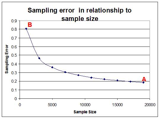
In the General Household Survey, the sample included 18,657 children of school going age for the whole of South Africa. This sample was intended to represent approximately 8,242,044 children of school going age in the total South African population. Because it is a sample there will be some degree of error in the results. However the sampling error in this case approaches a very respectable 0.2% (See point A in the graph above) because of the large sample size.
What does this mean? Well, if we are reporting values for a parameter - e.g. the number of children that are in school - and find that the result for the sample is 97.5%, it means that the same parameter in the population – the number of children that are in school - will range between 97.3% (97.5%-0.2%) and 97.7% (97.5%+0.2%). Note that if the sample included only 1000 people that the sampling error would have increased to 0.8%.
Statistical significance
It is not always correct to manually compare averages and percentages when one is interested in differences between different years’ or different provinces’ results. Percentages and averages are single figures that do not always adequately describe the variance on a specific variable. One needs to be convinced that a “statistically significant” difference is observed between two values before one can say one value is “better” or “poorer” than the other.
In order to make confident statements of comparison about averages, one would need to conduct tests of statistical significance (e.g. a t-test) using an applicable software package. These tests take into account the variance attributable to the sampling error and the normal variance around a mean. A person with some skills in statistical analysis could produce results (In a statistical analysis package or even in a spreadsheet application such as excel) that will allow adequate comparison of means between and within groups.
Weighting
Earlier we mentioned that one of the properties that influence representivity of sample results is whether the people all have the same probability of selection. If one had a complete list of all people in South Africa and a specific address for each one of them, you could have randomly selected people from this list and visited each one of them at their address. In this scenario each person has an equal chance to be included in the sample because you have the relevant details about them.
Unfortunately, researchers rarely have this kind of list and the costs would be very high if you had to visit each of the people you selected at their own address – You would probably end up speaking to one person per address only. To save time and money researchers rather speak to all people in a specific household that they select, but then all of the individuals in the population no longer have the same likelihood to be selected because this is impacted by which households are selected.
The probability of selection is even further complicated if one considers that researcher also don’t have a list with all households in South Africa to randomly select from. To get around this problem they use information about neighbourhoods and geographic locations to identify areas in which they will select households. When a survey uses neighbourhoods or households as a sampling unit, there is little control over the number of persons that will be included in the survey. One household in area A could have 5 people in it and the household next door might have 3 people in it. In order to ensure that the individuals within households (and households within neighbourhoods or household sampling units) are not disproportionately represented in relationship to known population parameters, weighting is applied.
Different weighting procedures can be used to correct for the probability of selection. The weighting procedure is usually selected by statisticians involved with the sampling in the survey. The weight to apply to each individual is usually captured as a variable somewhere in the dataset. Although it is beyond the scope of this manual to explain different ways of weighting it is important to consider that weighting will affect the percentages and absolute numbers produced.
The following table indicates how the percentage of 7 – 14 year olds that indicate they attend school in the General Household Survey differ when weighting is applied and when it is not applied.
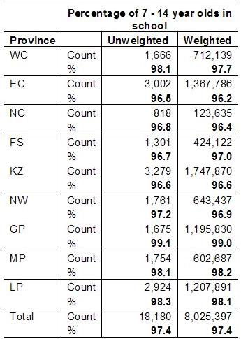
When analysing the data, it is important to ensure that the weighting is taken into account – both when percentages, averages and absolute numbers are computed. It is necessary to use a statistical analysis programme such as SPSS™ or STATA™ to produce any results.
------------------------------------
Attachment two: Household Survey Sampling Approaches
(This was produced by Khulisa Management Services)
For each of the three cities, Khulisa first conducted a purposive geographic sample, to be in alignment with the racial population and Living Standard Measure (LSM) levels three to seven[1] of the geographic area. LSM is used as an indicator of the principle index of the South African consumer market. It was first developed in 1991 by the South African Advertising Research Foundation (SAARF).
For each racial cell in the sampling framework above, the following methodology was used. Four by four, uniform grids were placed over the selected geographic areas. Cells from these grids were randomly selected and a subsequent ten by ten grid placed over the selected cell. A cell from the ten by ten grid was randomly selected after which a street block was selected. A street intersection was noted, and a house was randomly selected (left-side and out of ten houses on the block). The street intersection was the starting point as you move down the street/block. The primary sampling site was located on the left side of the street, with the alternative site being located on the right side of the street. The location of the two primary houses and two replacement houses was given to each fieldworker. This equated to 1200 sample sites and 1200 replacement sites picked from 600 street blocks. This strategy ensured that two fieldworkers – male and female – can work in the same street thus improving the safety levels of the fieldworkers, especially the females.
In an area with apartment buildings (like Joubert Park), after picking the apartment building the fieldworkers were instructed to select the second floor and the number indicated on the instructions for the flat to carry out the interviews.
If there was no house or flat in the pre-selected location, then it was recorded as an Unfeasible Site on the Fieldworkers’ Instrument Control Sheet. Similarly, if there were no eligible respondents in the household, then that was recorded as ALL Ineligible Respondents on the control sheet.
[1] The SABC ConsumerScope (2003) characterizes LSM levels three through seven by the following average monthly household income levels: Level 3: R1104; Level 4: R1534; Level 5: R2195; Level 6: R3575 and Level 7: R5504.